Preface
This is my project report for Bilkent University Cs-529 Dynamic and Social Network Analysis course. The report was originally in ACM journal format which is accessible through this PDF link. I just published it here as a blog post. The code, paper and slides are hosted on this repository.
Abstract
We propose a method to convert discrete genre labels to a continuous vector where each value shows the effect of a genre on the movie. This study explains how a bipartite rating graph can be transformed to input the topic-specific Pagerank algorithm to calculate continuous weights for each genre. Details on the selection of edge weight function and statistical adjustments to overcome the genre-imbalance problem are given. Results on a movie rating dataset show that the proposed method successfully calculates genre vectors of movies.
1. Introduction
Genre is defined as a particular style characterized by certain features in a movie, book, or other works of art. For example, the action genre is associated with its high emphasis on fights, explosions, special-effect and stunt work. The genre label of a movie is a set of genres that show the preeminent features in the movie. It's an important piece of information for movies because it roughly summarizes a movie with a handful of words. Therefore, there are many works based on genre analysis in the literature.
Some studies focus on finding genre labels of movies. Since correctly labeling a movie increases the marketing value of the movie, movie genre classification is a popular research area, especially in the machine learning field. Most studies do this classification task by finding patterns between the content of the movies and genre labels. For example, studies [1, 3, 14] try to predict the genre label of a movie by analyzing its script with NLP techniques. Studies [15, 17, 20] on the other hand, uses video clips of the movies to make genre predictions. This type of scene genre classification gained substantial popularity in recent years with the success of deep learning approaches in image/video classification tasks.
Genre labels play a significant role in recommendation systems as well. Movie recommendation systems try to predict which movies a user will like based on the attributes present in movies that were highly rated by the user previously. These attributes may include writers, directors, actors, language, and most importantly, genre labels of movies. Studies [13, 16] use genre labels of movies and rating matrix, which shows individual ratings given by viewers to movies, to produce movie and user profile vectors. This type of recommendation is known as content-based movie recommendation in the literature. They recommend movies by checking the similarity between movie profile vectors and viewer profile vectors. It is crucial to have accurate genre labels for this type of recommendation system.
The mentioned studies and many others suggest that genre labels are essential in any type of movie analysis. Traditionally, Genre labels of a movie are represented as a set of genres, which will be referred to as discrete labeling here and thereafter. A genre either exists or not in discrete labeling. This type of representation brings some problems. For example, if a movie is categorized as a horror movie, does it mean that the movie does not contain any elements from other genres? It probably does, but effects of other genres may be smaller than horror elements, so they are neglected in the labeling process. Also, if genre labels of a movie are comedy and action, discrete labeling doesn't allow us to distinguish which genre is more dominant in the movie. In this study, we propose a graph-based solution to calculate continuous vector representation of movies' genres (genre vectors) by using discrete labeling of movies. The continuous vector representation of a movie's genre is a \(d\)-sized real-valued vector. \(d\) is the number of genres in the system. The magnitude of each number in the vector shows the effect of a particular genre on the movie, and the sign shows the direction of this relationship. We believe this representation can help many computational movie analysis areas like recommendation systems as it carries more information about movies than the traditionally used discrete labeling.
We utilize the rating matrix to calculate the continuous vector representation of the movies. The rating matrix \(\mathbf{R}\) is a scarce \(m \times n\) matrix in a system with \(m\) users and \(n\) movies. Each entry \(r_{ij}\) shows the rating value of movie \(j\) given by user \(i\). We can regard this matrix as a 2-mode bipartite graph where users are one set and movies are the other set. An entry \(r_{ij}\) constitutes an edge between user node \(i\) and movie node \(j\). We apply the Topic-specific Pagerank algorithm to calculate genre vectors after transforming this graph into another graph that shows how much a movie influence other movies.
The rest of the paper is organized as follows: Section 2 gives a background on algorithms that are related to our proposed approach. Our methodology on formulating the problem as a topic-specific Pagerank problem is explained in Section 3. Section 4 describes our experiment setup and gives results. Finally, Section 5 concludes the paper.
2. Background
One way to formulate the described problem is to consider it a community detection problem. Community detection algorithms groups nodes into communities such that nodes in a community are densely connected. In our problem, each genre label represents a community. A movie may belong to more than one genre. It is known as overlapping community detection [12] in the literature. Another characteristic of our problem is that a movie's membership to a community (genre) is not binary. Instead, we would like to see a continuous value showing the strength of the movie's membership to a community. This kind of problem where each node belongs to each community to a different extent is known as fuzzy overlapping community detection [6]. Another different aspect of our problem is that we start with some labels. We have some initial beliefs on the membership of movies to genres, given as discrete labels. A similar feature is present in Label Propagation Algorithm (LPA) [21]. Label Propagation Algorithm is a semi-supervised technique to label unlabeled nodes in a graph by using a set of labeled nodes. In each iteration of the Label Propagation Algorithm, the label of each node is selected as the label that contains a maximum number of its neighbor nodes. This approach cannot solve our problem without modifying the algorithm because movies may have multiple labels and the movie-label relationship is not binary in our problem.
There are some studies that solve fuzzy overlapping community detection problems with ideas similar to Label Propagation Algorithm. NI-LPA [4] sort nodes in advance to overcome the instability problem of LPA caused by its random update order. LPANNI [11] adopts a similar node-sorting idea to find overlapping communities with better stability and accuracy. BMLPA [18] applies a two-step algorithm such that completely overlapped communities are removed in the second step, which is important when the number of communities is now known beforehand. However, none of these approaches can model our problem exactly.
Another way to approach the problem is viewing continuous genre values as popularity scores. And these popularity scores may be propagated between similar movies. Pagerank algorithm [2], initially proposed to find relevant websites for search queries, can be used to propagate these score values. The core ideas are as follows: if website A has a link to website B, website A conveys some of its importance score to website B. The amount of propagated importance score is inversely proportional to the number of outgoing links of website A. If we continue doing these score propagation operations until convergence, we can calculate the importance of every website. If we think world wide web as a directed graph \(G\), the score propagation in an iteration can be shown as:
Here \(Rank^{i}(u)\) denotes the score of node \(u\) in iteration \(i\). \(in\_adj(u)\) and \(out\_adj(u)\) denote incoming neighbors and outgoing neighbors of node \(u\) respectively. In the random surfer model, these values represent the probability of a random surfer going from one node to another. Pagerank also introduces a parameter \(\alpha\), which controls the probability that the surfer randomly jumps to another node instead of following the directed edges.
Although the original Pagerank algorithm is proposed on unweighted graphs, it is not difficult to see that the algorithm can be applied on weighted graphs by modifying the denominator inside the rank formula. The study [19] explores the idea of weighted Pagerank and compares it with the standard Pagerank algorithm in terms of relevancy of returned pages.
Topic-specific Pagerank [10] improves the Pagerank idea by making a biased jump decision with \(\alpha\) probability. Instead of jumping a random node with equal probability, the random node is selected, not necessarily uniformly, from a subset of nodes, known as topic nodes. This minor tweak in the algorithm allows us to calculate different Pagerank values depending on the search context. For example, if the search context is "news", the search engine can bring pages with high Pagerank values for the "news" topic.
TrustRank [8] is a variation of Topic-specific Pagerank to combat spam farms. In this algorithm, random jumps are biased in favor of trusted pages. So, pages linked by trusted pages have relatively high TrustRank scores. They compare TrustRank scores of the pages with their Pagerank scores to predict if a page is a spam. In particular, pages with a high Pagerank score and low TrustRank score have a decent chance to be spam pages.
3. Methodology
This section describes how the problem can be solved with the Topic-specific Pagerank algorithm. The first step of our approach is generating "the movie influence graph". The movie influence graph is a directed graph with \(n\) nodes. Each node represents a movie in the system, and each edge \((u, v)\) indicates that movie \(u\) influences movie \(v\) to some degree. The graph is constructed from the bipartite rating graph. We first give construction steps for the movie influence graph without assigning any weight to the edges here, and the following subsection discusses the edge-weight calculation alternatives.
The movie influence graph has an edge from node \(u\) to node \(v\) if node \(u\)'s user neighbors intersect with node \(v\)'s user neighbors in the rating graph. Since this construction rule is symmetric for \(u\) and \(v\), the generated directed graph has the reciprocity of 1. Here, it may be argued that representing this network as an undirected graph can be an option because of the full reciprocity. However, we decided to use the directed graph format since it gives us more freedom in the implementation. The directed graph representation allow us to assign different weights to edge \((u, v)\) and edge \((v, u)\). Also, if we want to control the density of the graph, we can separately choose whether edges \((u, v)\) and \((v, u)\) are discarded from the graph.
We create \(d\) sets of nodes for teleportation sets, where \(d\) is the number of genres. Each set \(C_i\) contains nodes initially labeled as genre \(i\). These sets are the teleportation locations for genre-specific Pagerank scores. For example, we're trying to find score values for genre \(i\). We run the Pagerank algorithm on the movie influence graph, but when the random surfer jumps with \(\alpha\) probability, instead of a random node in the whole graph, it jumps to a node in \(C_i\). We repeat this procedure for each genre. Finally, we calculate the genre scores of any movie by considering its genre-specific Pagerank scores and its traditional Pagerank score. The discussion for this final calculation is postponed to Section 4.
Another interesting aspect is the \(\alpha\) parameter. It is usually said that values around 0.15 give good results for the worldwide web. However, many factors affect the correct value of \(\alpha\) as discussed in [5]. In our problem, \(\alpha\) has another meaning. It controls how much trust we put into the initial labels of the movies. Let's consider two edges that \(\alpha=0\) and \(\alpha=1\) for comedy genre-specific Pagerank. When \(alpha\) is 1, the random surfer teleports to a random movie that is initially labeled as comedy. It doesn't visit other nodes at all. For this reason, the movies will have 0 Pagerank scores for genres that are not in their genre sets. On the other end, if \(\alpha\) is 0, the algorithm doesn't consider teleportation sets. The random surfer never teleports. As a result, genre Pagerank scores for a movie will be the same for all genres. A value between 0 and 1 indicates that we trust initial labels to an extent but also, we let the algorithm change our trust by using the movie influence network. \(\alpha\) value should be tuned carefully to get the desired result.
3.1 Edge Weight Assignment
Although the rating matrix has rating values for the edges, we didn't use the rating values in the weight assignments. We believe ratings don't give strong indications about genre influence between movies. So, we regard the rating graph as an unweighted graph. In other words, the rating graph is converted into the "who watched what" graph.
We consider several formulas to calculate the weight between node \(u\) and \(v\), \(w(u, v)\), for every \(u\), \(v\) pair in the edge set of the movie influence graph. The first formula given below calculated the number of users who watched both movies. The adjacency matrix using this formula can be calculated by multiplying the adjacency matrix of the bipartite rating graph with its transpose and setting the diagonals 0 to avoid self-loops. The main problem with this formula is that it gives very large weights between popular movies. This results in popular nodes ignoring unpopular nodes in the Pagerank calculations. However, many uncommon movies are heavily influenced by classic popular movies in real life, so this calculation doesn't entirely model the behavior we expect from the movie influence graph.
Jaccard and Sørensen's similarities, listed below in order, are considered as alternatives. They mitigate the mentioned problem by normalizing the values with respect to the size of nodes' adjacency lists. However, the same problem still exists to some extent.
To be able to solve the mentioned issue, if the the size of adjacency list of node \(u\), \(|adj(u)|\), (popular movie) is much larger than node \(v\)'s (unpopular movie) size of adjacency list, it is better for the weight formula for \(w(u, v)\) to not contain \(|adj(u)|\). Two such weight formulas obeying that statement are given below. The first equation (\(w_4\)) basically divides the number of people that watched both movies by the number of people that watched the movie targeted by the edge to get the weight of the edge. It is the only function described here that is not symmetric. This asymmetric behavior can be a desired property since the Pagerank scores in undirected graphs tend to correlate with degree centrality [7] strongly. However, the manual inspection on a small subset of the dataset didn't give promising results in our experiments. Therefore, we decided to use \(w_5\) weight calculation in our study.
In the \(w_5\) weight calculation, the denominator is replaced with \(min(|adj(u)|, |adj(v)|)\). Here, \(w_5\) gives higher weight values for edges going from unpopular movies to popular movies compared to \(w_4\). For this reason, it may be argued that unpopular movies propagate more significance than they should. However, We should note that the Pagerank values of unpopular movies are already low. So, although these edges have high weights, they don't affect target nodes much. It might be why we couldn't get meaningful results with the \(w_4\) weight formula since it penalizes unpopular movies twice.
4. Experiment Setup and Results
4.1 Datasets
We use movielens-25m [9] dataset which contains 25,000,000 ratings given by over 160,000 users to around 60,000 movies.
Some statistics of movielens-25m are given in Table 1.
Our bipartite rating graph consists of users, movies, and rating pairs between users and movies.
It can be considered a sparse graph due to its low 0.0026 density.
Differences between highest degree nodes and lowest degree nodes in both user and movie nodes are significantly large.
% We also generated a dataset using TMDb API (developers.themoviedb.org).
% This dataset includes basic information about movies like actors, titles, writers, poster images, and genres. Genres from this dataset are used to create topics for the topic-specific Pagerank algorithm.
| Property | Value |
|---|---|
| Number of users (rows) | 162,541 |
| Number of movies (columns) | 59,047 |
| Number of ratings | 25,000,095 |
| Density | 0.00260 |
| Minimum rating | 0.5 |
| Maximum rating | 5.0 |
| Minimum row degree | 20 |
| Maximum row degree | 32,202 |
| Average row degree | 153.80 |
| Minimum column degree | 1 |
| Maximum column degree | 81,491 |
| Average column degree | 423.39 |
Table 1. Properties of movielens-25m dataset
Figure 1 shows the degree distributions of user and movie nodes. The linearity in this log-scaled figure suggests that user and movie nodes' degrees follow a power-law distribution. As seen in the figure, more than 10,000 movies have a viewer count of 1. The frequency of movies drops quickly as their degrees increase. We can say that a large subset of users watches a small subset of movies. Similarly, a small subset of users watched a large subset of movies.
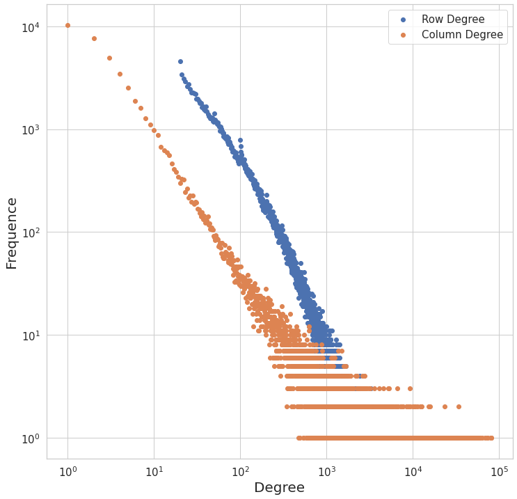
Figure 1. Degree-Frequence plot of rows (users) and columns (movies) in log scale
The dataset also includes genre information. Each movie is associated with at least one genre of out 19 genres. These genres are drama, comedy, thriller, romance, action, horror, documentary, crime, adventure, science-fiction, children, animation, mystery, fantasy, war, western, musical, film-noir, and IMAX. Figure 2 shows the count of movies with mentioned genres. The figure shows that the drama genre is the largest one, appearing in more than 25000 movies. The least number of movies are observed in IMAX and film-noir movies. Also, these two categories do not quite fit our definition of genre. For these reasons, we removed IMAX and film-noir from the dataset. Also, it is difficult to assign a continuous value for animation and documentary categories. For example, a movie is either a documentary or not. It doesn't make sense to assign a real-valued number for these categories. Therefore, documentary and animation genres are also dropped from the dataset. With these changes, the total number of genres in the dataset is reduced to 15.
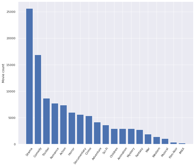
Figure 2. Histogram of genres
4.2 Results
The movie influence graph constructed according to the steps mentioned in Section 3 has 1,364,630,530 edges. This number is quite large from a computational perspective. We removed some unimportant parts of this graph to run the Pagerank algorithm faster. The edge weight frequency plot shown in Figure 3 gives us some hints about which edges to remove. The figure shows that the huge portion of the edges has suspiciously 1.0, 0.5, 0.33, or 0.25 weights. When these edges are investigated, it turns out that most of the edges with 1.0, 0.5, 0.33, and 0.25 weights belong to movies with 1, 2, 3, and 4 view count. We give an example to show why this result is expected. Suppose that a user watched 10,000 movies, and one of those movies is watched only by this user. It means there is an edge with weight 1 between that movie and other movies because of a single view of the movie. Although those edges are very important for the movie with 1 view count, the movie itself is not important for our analysis. Therefore, we decided to remove all movies with a low view count. When we removed the movies with less than 15 view count, We reduced our total number of movie nodes to 20,034.
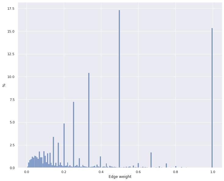
Figure 3. Weight distribution of \(w_4\) weight calculation
Figure 4 shows the weight distribution of reduced set of 20,034 movies. Most edges have low weights, and almost no edge has a weight of 1. This is a more expected edge weight distribution for a movie influence graph. As seen in the figure, more than 80\% of edges have less than 0.2 weights. Since weights represent the influence between movies, low scores mean low influence. So, we removed all edges having less than 0.2 to reduce the edge count even lower. The idea is to remove most edges without affecting Pagerank scores much by removing the low-impact edges. After this removal, we get a movie influence graph with around 20,000 nodes and 56,000,000 edges. Then, we run the Pagerank algorithm on the graph.
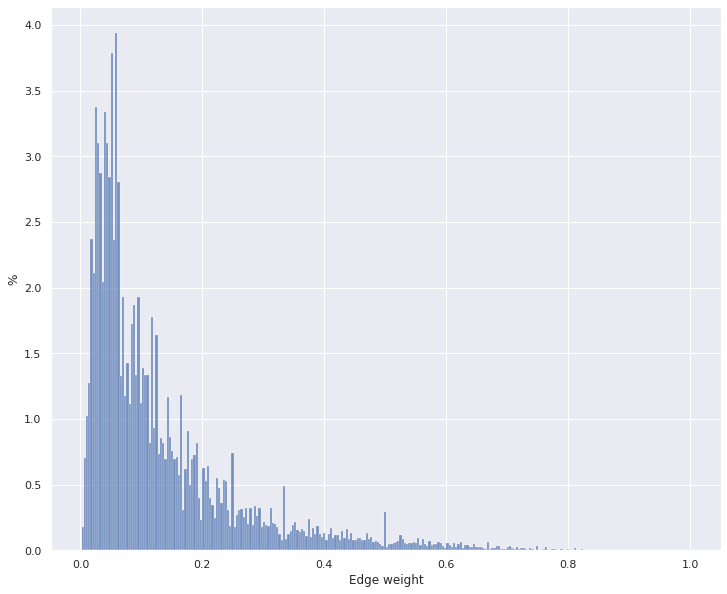
Figure 4. Weight distribution after vertex/edge cleaning
It is observed that the imbalance of movie counts between different genres as observed in Figure 2 has a negative effect on the Pagerank values. This imbalance makes the genre Pagerank values of a movie difficult to compare. To solve this issue, we adjusted the \(\alpha\) parameter with respect to the movie count of each genre. This adjustment is made in a way that teleporting to a horror movie in horror-specific Pagerank has the same probability as teleporting to an action movie in action-specific Pagerank.
Here, we explain how we calculate the genre score of a movie using Pagerank scores. Let \(score_g(u)\) denote the score of movie \(u\) for genre \(g\) and let \(PR(u)\) and \(PR_g(u)\) respectively denote the traditional Pagerank score of node \(u\) and Pagerank score of node \(u\) for genre \(g\). The equation for \(score_g(u)\) is given below.
\(E[PR_g(u | PR(u)]\) is the expected \(g\)-genre Pagerank value of a movie with \(PR(u)\) Pagerank score. This expected value is computed by fitting all movies' Pagerank scores to their genre-specific Pagerank scores with a least square regression. So, if \(score_g(u)\) is a positive number, we can say that genre \(g\) affects the movie \(u\) in a positive way. The magnitude of the number shows the extent of this influence. On the other hand, negative values or values close to 0 indicate that genre does not influence the movie or the influence is negligible.
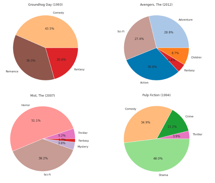
Figure 5. Genre pie-chart of the 4 movies. Top-left: Groundhog Day, Top-right: Avengers, Bottom-left: The mist, Bottom-right: Pulp fiction
Figure 5 shows a pie-chart plot of positive genre scores for a sample of movies. In the top-right part of the figure, we see the values for the Groundhog Day movie. In the dataset, the movie is labeled comedy, romance, and fantasy. We can see the influence of each genre easily in the figure. Comedy is the most, and fantasy is the least dominant genre for this movie. We can say that the genres not listed in the initial genre set have no significant impact for this movie. However, this is not the case for the other movies. Scores of horror, sci-fi, thriller, fantasy and mystery genres for the movie Mist are shown in the figure's top-left part. The movie's initial genre labels do not contain thriller, fantasy, or mystery. We can see that our proposed method also finds the relationships that are not in the original labeling of the movies.
4.3 Limitations and Future Work
Even though the model is quite successful at comparing scores of different genres in a movie, unfortunately, it is not as good at comparing different movies. Figure 6 may provide an insight into the cause of this problem. Each point represents a movie in the plot where the x-axis shows the Pagerank score, and the y-axis shows the action genre score calculated as explained in Section 4.2. As Pagerank scores decrease, the action genre scores diverge. Similar patterns are observed in all other genres as well. This pattern makes it difficult to compare genre scores of movies that greatly differ in Pagerank. We need to investigate the structure of the influence graph and the effect of weight function on the structure to understand the root of the problem. We guess the issue can be solved with a more proper weight function and correct statistical adjustments. Since required experiments exceed the scope of the project, we end our analysis here.
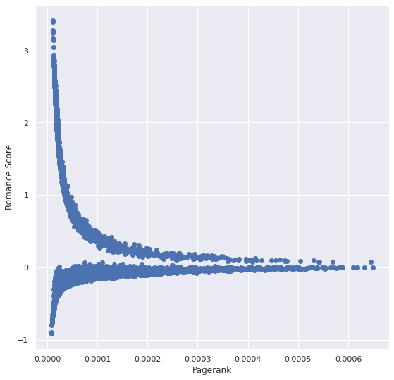
Figure 6. The problem of score divergence
Because of this problem, we couldn't do experiments to understand the model's predictive power. Our initial plan was to compare the model's accuracy with a simple Naive-Bayes model. The planned comparison workflow was as follows. Firstly, labels of a random sample of the movies are removed from the dataset. These movies constitute our test set. For each movie in the test set, we pick \(k\) genres with top scores where \(k\) is the size of the movie's genre set. Then, we check how many predicted labels match the initial labels. We calculate the correctly predicted label count for the proposed Pagerank model and a basic Naive-Bayes model. And, finally, we compare the results.
5. Conclusion
We proposed a method to convert discrete genre labels of movies into continuous vectors. We showed how a rating graph could be converted into a movie influence graph, which becomes the input of topic-specific Pagerank to calculate scores for each genre. The implementation details of weight calculation on movie influence graph and statistical adjustments to solve the imbalanced genre problem are explained. We showed that the proposed method gives promising results for labeled and unlabeled genres.
References
- Alex Blackstock and Matt Spitz. 2008. Classifying movie scripts by genre with a MEMM using NLP-Based features. Citeseer (2008).
- Sergey Brin and Lawrence Page. 1998. The anatomy of a large-scale hypertextual web search engine. Computer networks and ISDN systems 30, 1-7 (1998), 107–117.
- Pratik Doshi and Wlodek Zadrozny. 2018. Movie genre detection using topological data analysis. In International Conference on Statistical Language and Speech Processing. Springer, 117–128.
- Imen Ben El Kouni, Wafa Karoui, and Lotfi Ben Romdhane. 2020. Node Importance based Label Propagation Algorithm for overlapping community detection in networks. Expert Systems with Applications 162 (2020), 113020.
- David F Gleich, Paul G Constantine, Abraham D Flaxman, and Asela Gunawardana. 2010. Tracking the random surfer: empirically measured teleportation parameters in PageRank. In Proceedings of the 19th international conference on World wide web. 381–390.
- Steve Gregory. 2011. Fuzzy overlapping communities in networks. Journal of Statistical Mechanics: Theory and Experiment 2011, 02 (2011), P02017.
- Vince Grolmusz. 2015. A note on the pagerank of undirected graphs. Inform. Process. Lett. 115, 6-8 (2015), 633–634.
- Zoltan Gyongyi, Hector Garcia-Molina, and Jan Pedersen. 2004. Combating web spam with trustrank. In Proceedings of the 30th international conference on very large data bases (VLDB).
- F Maxwell Harper and Joseph A Konstan. 2015. The movielens datasets: History and context. Acm transactions on interactive intelligent systems (tiis) 5, 4 (2015), 1–19.
- Taher H Haveliwala. 2003. Topic-sensitive pagerank: A context-sensitive ranking algorithm for web search. IEEE transactions on knowledge and data engineering 15, 4 (2003), 784–796.
- Meilian Lu, Zhenglin Zhang, Zhihe Qu, and Yu Kang. 2018. LPANNI: Overlapping community detection using label propagation in large-scale complex networks. IEEE Transactions on Knowledge and Data Engineering 31, 9 (2018), 1736–1749.
- Fragkiskos D Malliaros and Michalis Vazirgiannis. 2013. Clustering and community detection in directed networks: A survey. Physics reports 533, 4 (2013), 95–142.
- SRS Reddy, Sravani Nalluri, Subramanyam Kunisetti, S Ashok, and B Venkatesh. 2019. Content-based movie recommendation system using genre correlation. In Smart Intelligent Computing and Applications. Springer, 391–397.
- Amr Shahin and Adam Krzyzak. 2020. Genre-ous: The Movie Genre Detector.. In ACIIDS (Companion). 308–318.
- Gabriel S Simões, Jônatas Wehrmann, Rodrigo C Barros, and Duncan D Ruiz. 2016. Movie genre classification with convolutional neural networks. In 2016 International Joint Conference on Neural Networks (IJCNN). IEEE, 259–266.
- Mahiye Uluyagmur, Zehra Cataltepe, and Esengul Tayfur. 2012. Content-based movie recommendation using different feature sets. In Proceedings of the world congress on engineering and computer science, Vol. 1. 17–24.
- Jônatas Wehrmann and Rodrigo C Barros. 2017. Movie genre classification: A multi-label approach based on convolutions through time. Applied Soft Computing 61 (2017), 973–982.
- Zhi-Hao Wu, You-Fang Lin, Steve Gregory, Huai-Yu Wan, and Sheng-Feng Tian. 2012. Balanced multi-label propagation for overlapping community detection in social networks. Journal of Computer Science and Technology 27, 3 (2012), 468–479.
- Wenpu Xing and Ali Ghorbani. 2004. Weighted pagerank algorithm. In Proceedings. Second Annual Conference on Communication Networks and Services Research, 2004. IEEE, 305–314.
- Howard Zhou, Tucker Hermans, Asmita V Karandikar, and James M Rehg. 2010. Movie genre classification via scene categorization. In Proceedings of the 18th ACM international conference on Multimedia. 747–750.
- Xiaojin Zhul and Zoubin Ghahramanilh. 2002. Learning from labeled and unlabeled data with label propagation. (2002).
Comments